Comparative Study of Machine Learning Methods on Circle-In-Square and MNIST Tasks

March 9, 2025
Lloyd Watts

In 2025, Artificial Intelligence (AI) research and product development is dominated by Large Language Models (LLMs), which in turn are based on Auto-Regressive Decoder-Only Transformers, which are based on Deep Neural Networks (DNNs). DNNs are the dominant core component because they are powerful, universal function approximators with a well-defined learning rule (Back-Propagation), and their high performance and scalability to large and deep networks has led to a decade of industrial infrastructure development, in software (Pytorch, TensorFlow), and in hardware (GPUs with CUDA software development platform, multi-core CPUs).

But DNNs have a number of serious problems, including lack of interpretability/explainability, training requires multiple passes through the entire training dataset, no few-shot learning, and no on-line continuous learning without catastrophic forgetting. And there are other Machine Learning methods which have different/better properties: Bayesian Classifiers, Adaptive Resonance Theory (ARTMAP), Nearest Neighbor Classifier, Support Vector Machines, 2-Layer DNNs, Convolutional DNNs, DNNs with Neocortix Deep Attribution Network.

The purpose of this investigation was to compare all of the above Machine Learning methods on two familiar tasks: the Circle-In-Square Task and the MNIST Handwritten Digit Recognition Task. We measured their training time and test time on a 64-core CPU machine with 128 GB of RAM, and we created plots and visualizations of the data sets and the internal data representations and decision boundaries of each model, to illustrate why some models are explainable and some are not.

Training Datasets for the Circle-In-Square and MNIST Tasks

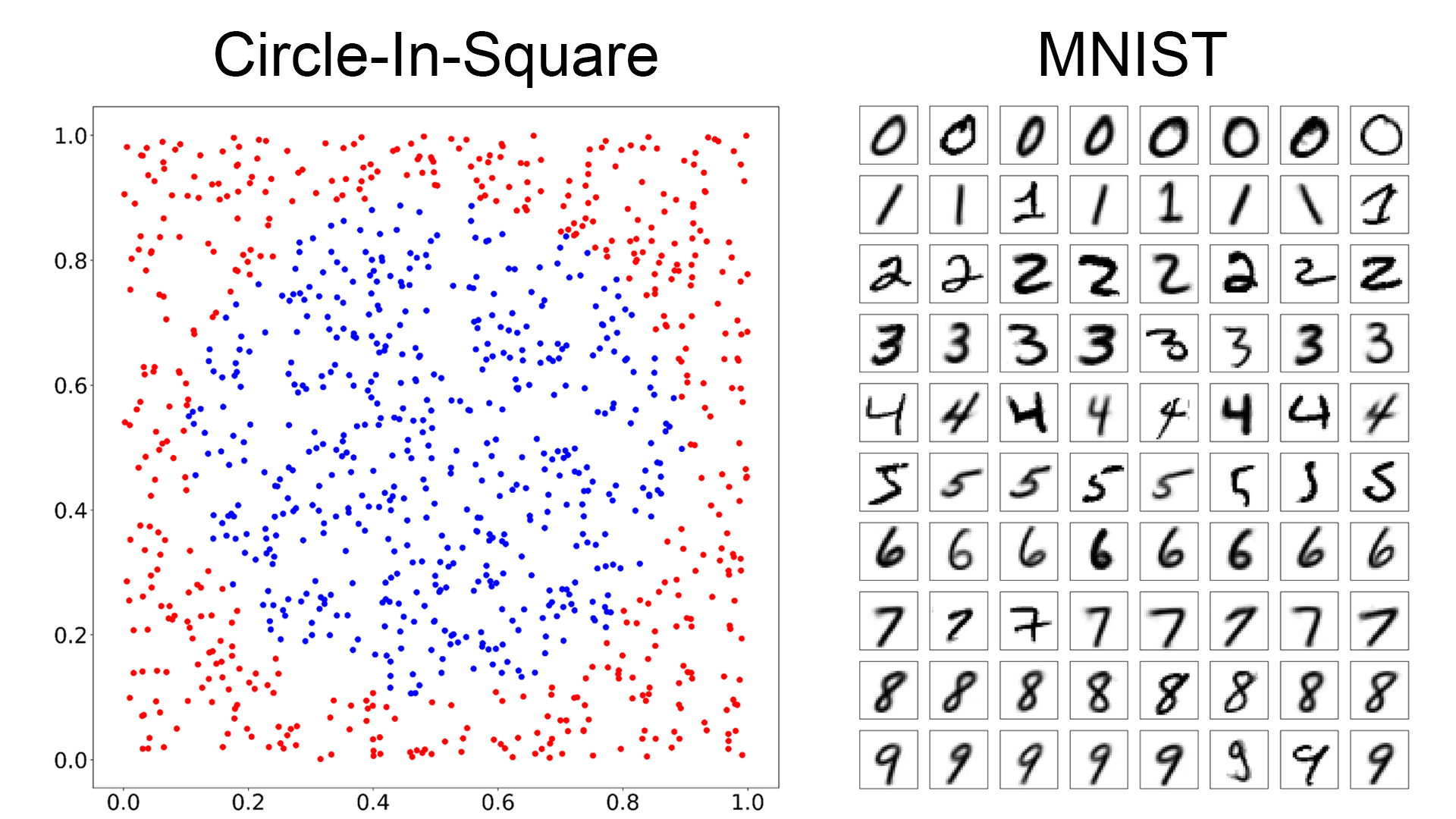
Figure 1: Training Datasets for the Circle-In-Square and MNIST Tasks. The Circle-In-Square dataset has 1000 data points, in two classes, in two dimensions. The MNIST dataset has 60,000 samples, in 10 classes (digits 0-9), in 28x28=784 dimensions. We're showing 8 representative samples for each class, above.

We are using the Circle-In-Square dataset because the whole dataset and any model's decision boundaries can be visualized easily. We are using the MNIST dataset because it is a well-known dataset which established Deep Convolutional Neural Networks as the best-performing model for image classification tasks, and thus it is a de facto standard reference for evaluating other models. But with 60,000 samples in 10 classes in 784 dimensions, it is a challenge to visualize the MNIST data and the model decision boundaries.

Summary of Results for the Circle-In-Square Task

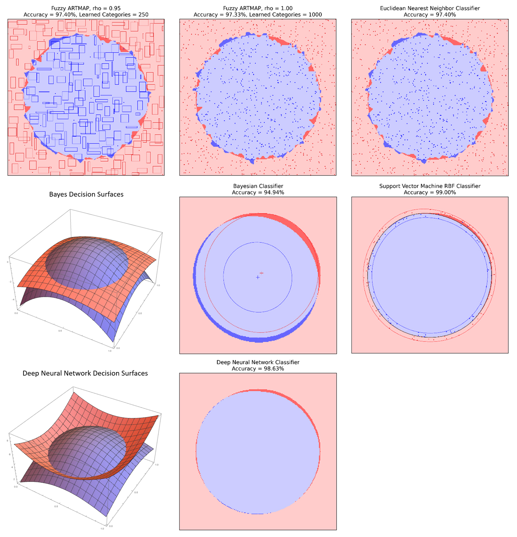
Figure 2: Model Results for the Circle-In-Square Task, for ARTMAP, Nearest-Neighbor, Bayesian Classfier, Support Vector Machine, and Deep Neural Network.

In Figure 2, we can see how the different models work, and what accuracy they can get.

• Fuzzy ARTMAP with Vigilance rho=0.95 gets accuracy=97.40% with 250 Learned Categories. This method has many desirable properties: It is inherently explainable, it can do single-pass learning, few-shot learning, on-line and continuous learning, with no catastrophic forgetting. In the figure, the small rectangles are the Learned Categories, which represent bounding boxes around groups of training samples. At training time, each new training sample is compared to all existing Learned Categories. If the new training sample is within a Manhattan Distance tolerance of an existing Learned Category, it is said to "resonate", and the Learned Category is updated to include the new training sample; otherwise, a new Learned Category is created to include the new training sample. Notice that this example there are 250 Learned Categories, with 1000 data points. So, on average, each Learned Category includes about 4 data point, and thus ARTMAP gets high classification accuracy=97.40% with a compression ratio of about 4:1. At test time, a new test sample is compared to all of the Learned Categories, and the class of the Learned Category with the smallest Manhattan Distance to the new test sample is chosen as the class of the new test sample. And now we can see why this is inherently explainable. If we are asked why a new test sample was assigned to a particular class, the answer is that it was most similar to this particular Learned Category of that class, and we can retrieve the corresponding Learned Category to back it up. This inherent explainability is a great strength of the Fuzzy ARTMAP method.
• Fuzzy ARTMAP with Vigilance rho=1.0 gets accuracy=97.33% with 1000 Learned Categories. This is the special case of rho=1.0 where every new training sample gets a new Learned Category, with no data compression (1:1). In this limiting case, Fuzzy ARTMAP is essentially equivalent to a Manhattan Nearest Neighbor Classifier.
• Euclidean Nearest Neighbor Classifier gets accuracy=97.40%. For the Circle-In-Square task, Euclidean and Manhattan Distance metrics perform about the same. Notice the irregular decision boundary for all three of the above examples. ARTMAP and Nearest Neighbor methods are based on local distance metrics, without any smoothing or regularization of the decision boundary.
• Bayesian Classifier gets accuracy=94.94%. The Bayesian Classifier computes the mean and covariance matrices for all the data in each class, and models each class with a Normal Distribution (Gaussian or Bell-shaped curve). This leads to the Bayes Decision Surfaces: a blue one with a taller, narrower peak, and a red one with a shorter, wider peak. This results in a smooth, regularized decision boundary. But the errors are fairly bad because the mean values (crosses in the figure) are slightly shifted from the correct value, since there are only 1000 data points.
• Support Vector Machine with Radial Basis Function Kernel gets accuracy=99.00%. This is the best-performing model on the Circle-In-Square task. This method only uses the data points that are close to the decision boundary (the Support Vectors), as shown in the figure. The RBF Kernel method results in a significant smoothing/regularization of the decision boundary, with a very good fit to the underlying distribution, resulting in a very high accuracy=99.00%.
• Deep Neural Network gets accuracy=98.63%. This is the second-best-performing model on the Circle-In-Square task. The DNN is a universal function approximator, and it uses its neurons and nonlinear activation functions to build up two decision surfaces, one for each class, as shown in Figure 2. The decision surface for Class 0 (points inside the circle) is colored blue, and it is a concave-down hump. The decision surface for Class 1 (points outside the circle) is colored red, and it is a concave-up bowl shape. The decision boundary is the nearly-circular closed curve where the red and blue decision surfaces intersect, and it is very good fit to the underlying distribution, resulting in a very high accuracy=98.63%.

But what is the relationship between the neurons and nonlinear activation functions and the two decision surfaces for the Deep Neural Network? Figure 3 shows the Pytorch code for this two-layer fully-connected neural network with 2 inputs (2D input vectors), 1700 hidden neurons, and 2 outputs (2 classes). It uses a Rectified Linear or ReLU() activation function, also shown in Figure 3. The 1D ReLU() function looks like a bent line. The 2D ReLU() function looks like a bent plane, with a crease line where the plane bends.

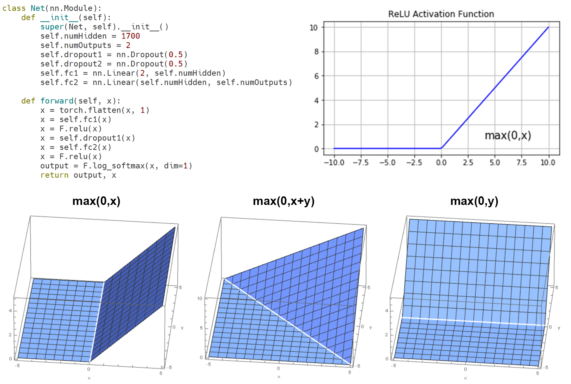
Figure 3: DNN Pytorch code and Rectified Linear ReLU() Activation Function in 1D (bent line) and 2D (bent planes with different rotations).

In Figure 4, we show that the sum of 4 bent planes can make a piecewise planar approximation to a smooth curved surface.

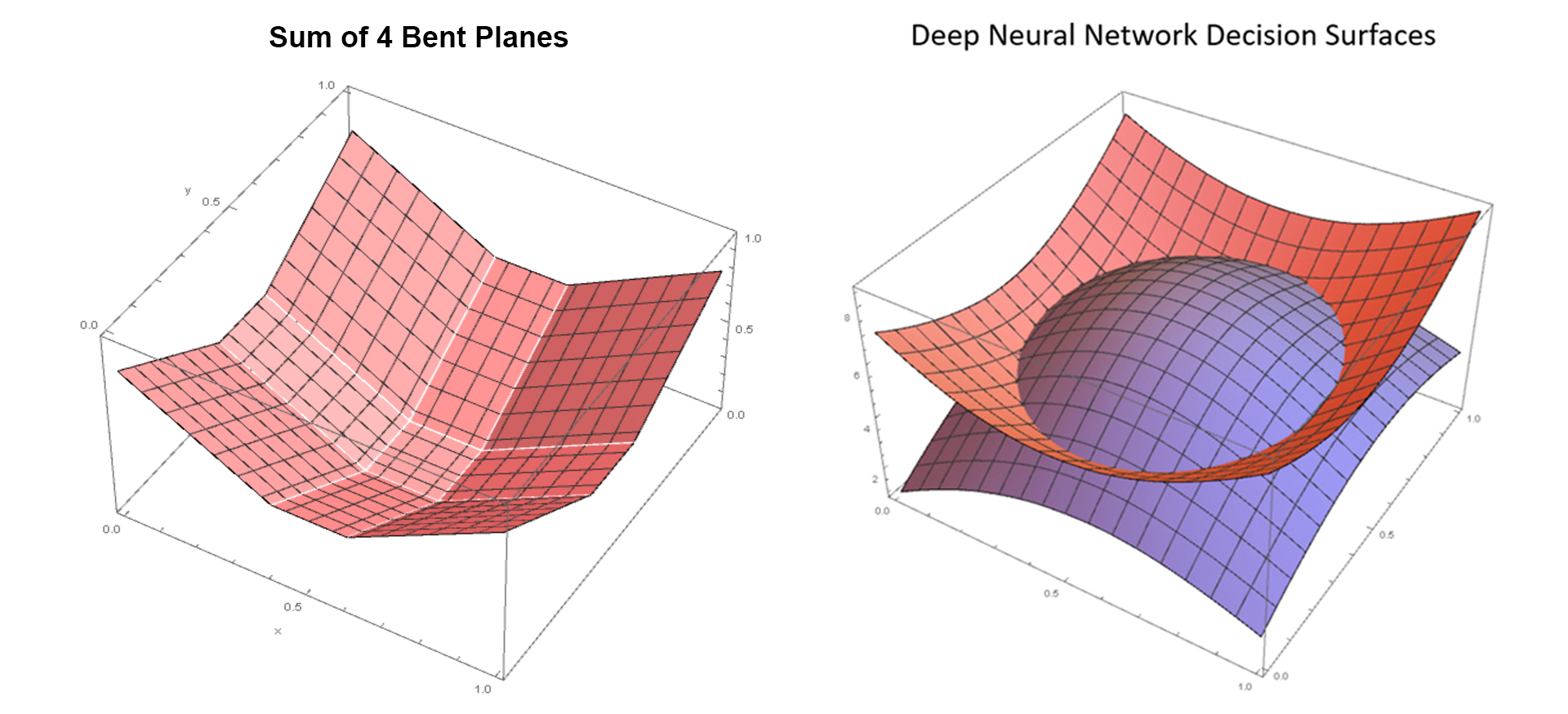
Figure 4: A tiny Neural Network with 4 hidden neurons can create 4 Bent Planes. The Sum of those 4 Bent Planes can make a piecewise planar decision surface.

In the Circle-In-Square example, each of the 1700 hidden neurons creates a bent-plane function, where the weights and biases of each hidden neuron determine the position and rotation of its bent-plane crease line. Figure 5 shows a plot of all 1700 of those bent-plane crease lines for Class 0 and Class 1. Bent-plane crease lines are drawn in shades of black for bending-down bent planes (negative weight in layer 2), and in shades of white for bending-up bent planes (positive weight in layer 2). And finally, all of these weighted rotated bent-plane contributions add up to make the two smooth decision surfaces. This illustrates how a DNN can be a universal approximator of smoothed curved surfaces, just using weighted sums of rotated bent planes.

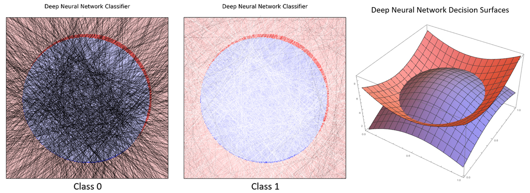
Figure 5: DNN individual neuron bent-plane crease lines, and the composite decision surfaces created from weighted sums of 1700 rotated bent planes.

Now we can see why Explainability/Interpretability of Deep Neural Networks is considered a difficult problem, even in a simple 2D problem like Circle-In-Square. Many weighted and rotated bent planes contribute to the height of a decision surface at any particular x-y position. With additional computational effort, often using auto-encoders, we can find out which neurons make the greatest contribution to a particular classification decision, and thus we can make some broad statements like "this neuron seems to be responsible for detecting this feature in the training data". But this is a challenging present-day research problem. Some of the best work in this exciting field is being done at Anthropic by Chris Olah and his Interpretability Research team.

Finally, we note that Deep Neural Networks are the dominant Machine Learning method, and yet they are not inherently explainable, so significant effort is going into finding ways to make them explainable (Anthropic Interpretability techniques, Neocortix Deep Attribution Networks). But we should remember that Fuzzy ARTMAP is also a high-performance Machine Learning method, and it is inherently explainable, because it carries representative training set data with the Learned Categories in its model representation.

Now that we have examined the different Machine Learning models on the simple 2D 2-class Circle-In-Square problem, let's look at the more complex 784-D 10-class MNIST problem.

Summary of Results for the MNIST Task

The MNIST Handwritten Digit task consists of 28x28-pixel images of 10 handwritten digits (0-9). There are 60,000 samples in the training set, and 10,000 samples in the test set. 8 representative training set samples in each of the 10 classes are shown in Figure 1.

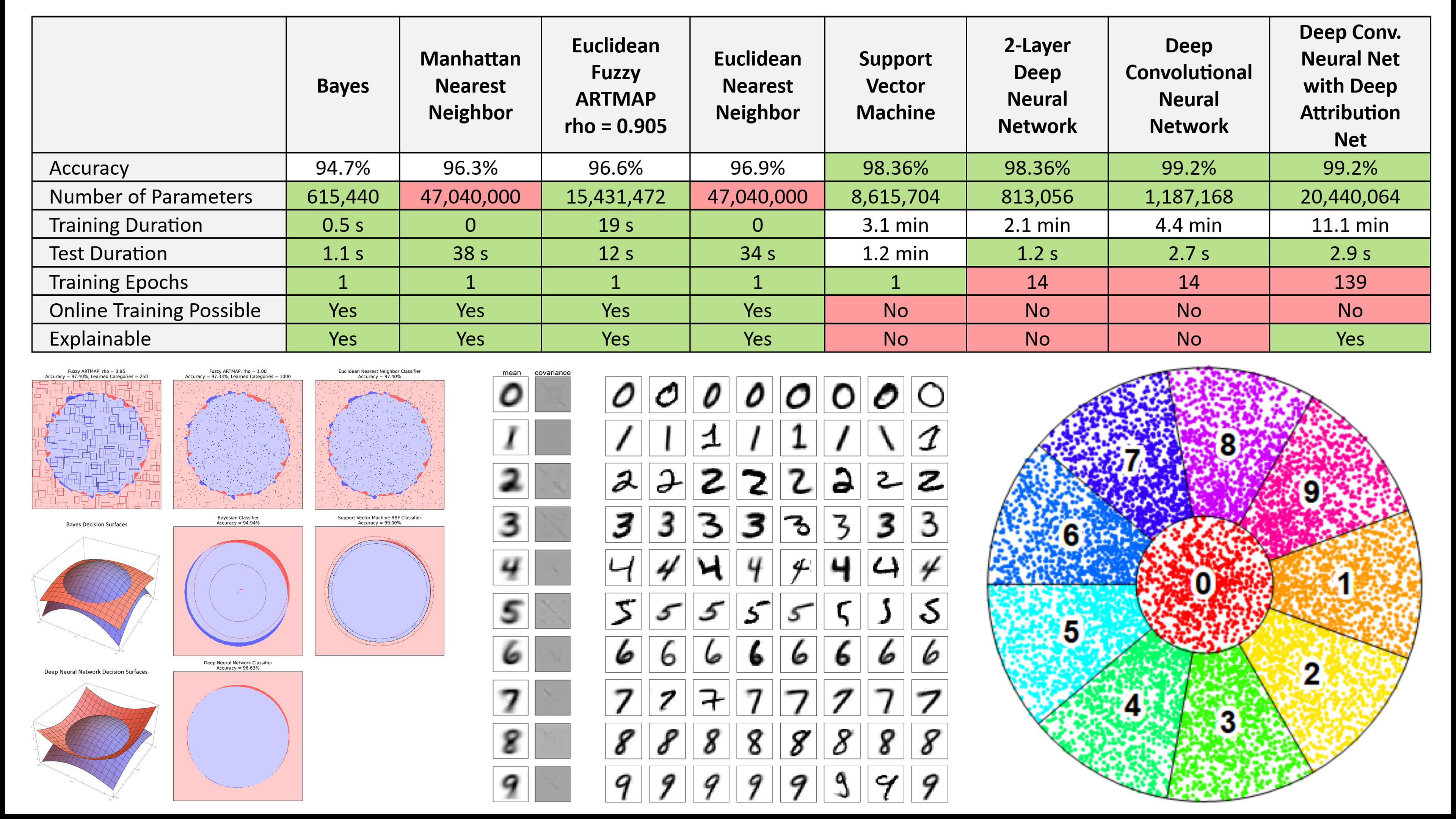
We used high-performance implementations of all of the above Machine Learning models, and evaluated them on their recognition accuracy, number of stored parameters in the trained model, training duration, test duration, number of training epochs (training passes through the training set), and binary judgment of on-line continuous learning, and inherent explainability. All of the Machine Learning models were trained and run on a 64-core CPU machine with 128 GB of RAM, with no GPU. A summary of all results is shown in Figure 6.

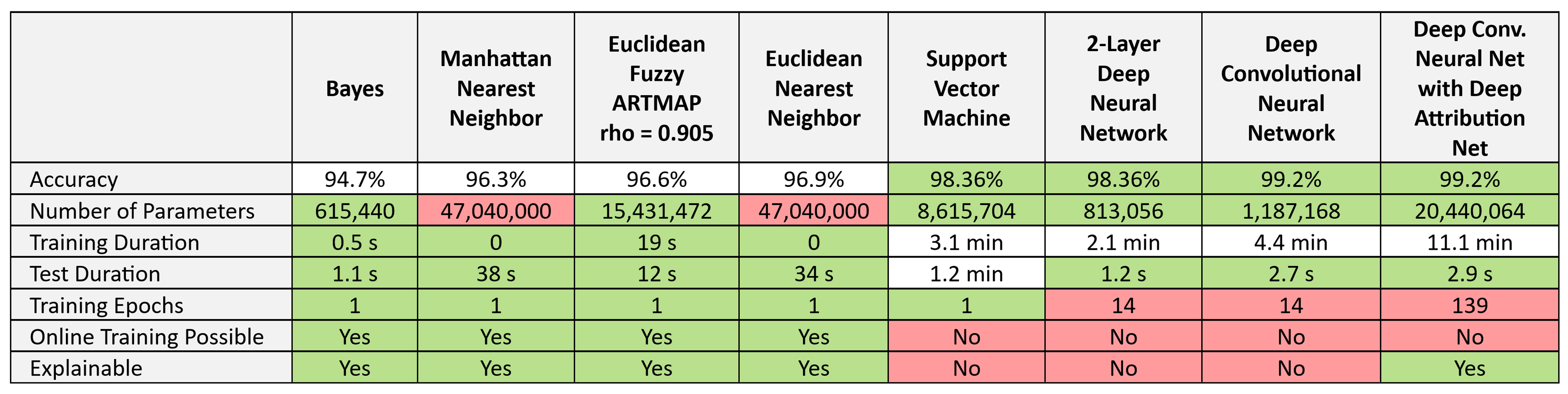
Figure 6: Model Results for the MNIST Task, for ARTMAP, Nearest-Neighbor, Bayesian Classfier, Support Vector Machine, and Deep Neural Network.

We can make some broad statements about the different models and their performance on the MNIST task:

• Accuracy: Deep Convolutional Neural Networks get the highest accuracy=99.2%. Of the models that are inherently explainable, Euclident Nearest Neighbor gets the highest accuracy=96.9%. Of the models that are inherently explainable which do not store the entire training set, Euclidean Fuzzy ARTMAP gets the highest accuracy=96.6%. Bayes gets the lowest accuracy=94.7%, because the per-pixel data distributions are not Gaussian-distributed, so the model is not a great fit for the data.
• Number of Parameters: Bayes has the lowest number of stored parameters=615,400, since it only stores the means and covariance matrices of the training dataset. 2-Layer Deep Neural Network and Deep Convolutional Neural Networks are also very efficient, with 813,056 and 1,187,168 stored parameters, respectively. Manhattan and Euclidean Nearest Neighbor are the least efficient, with both storing the entire training dataset of 60,000 x 784 = 47,040,000 parameters. The two high-accuracy explainable methods are Euclidean Fuzzy ARTMAP and Deep Convolutional Network with Neocortix Deep Attribution Network, with 15.4 Million and 20.4 Million parameters, respectively. Generally, explainable models require more storage than non-explainable models.
• Training Duration and Training Epochs: Manhattan and Euclidean Nearest Neighbors have zero training duration, because they simply store the entire training set. Bayes has extremely fast training duration (0.5s) in a single training epoch, because it only has to compute the means and covariance matrices. Fuzzy ARTMAP has very fast training duration (19s) in a single training epoch (but this fast training time was achieved with considerable effort, requiring a multi-threaded C++ implementation using AVX Intrinsics). Deep Convolutional Neural Network takes 4.4 minutes over 14 training epochs. Deep Convolutional Neural Networks with Neocortix Deep Attribution Network has the longest training duration of 11.1 minutes over 139 training epochs. High accuracy and Explainability come with a cost of long training times.
• Online Training: The models capable of Online Training (or Continuous Learning) are Bayes, Manhattan and Euclidean Nearest Neighbor, and Fuzzy ARTMAP. The models that are not capable of Online Training are Support Vector Machines and the Neural Network variations.
• Explainability: The Explainable models are Bayes, Manhattan and Euclidean Nearest Neighbor, Fuzzy ARTMAP, and Deep Neural Network with Neocortix Deep Attribution Network. The models that are not capable of Online Training are Support Vector Machines and the other Neural Network variations without Neocortix Deep Attribution Network.

Now, let us look closer at the individual models.

• Fuzzy ARTMAP with Vigilance rho=0.905 gets accuracy=96.6% with 19,683 Learned Categories. This method has many desirable properties: It is inherently explainable, since the Learned Categories are directly related to the training samples. It can do single-pass learning, few-shot learning, on-line and continuous learning, with no catastrophic forgetting. It is fast to train (19 seconds) in a single training epoch, using a multi-threaded C++ implementation using AVX Intrinsics. Examples of ARTMAP Learned Categories on MNIST are shown in Figure 7.

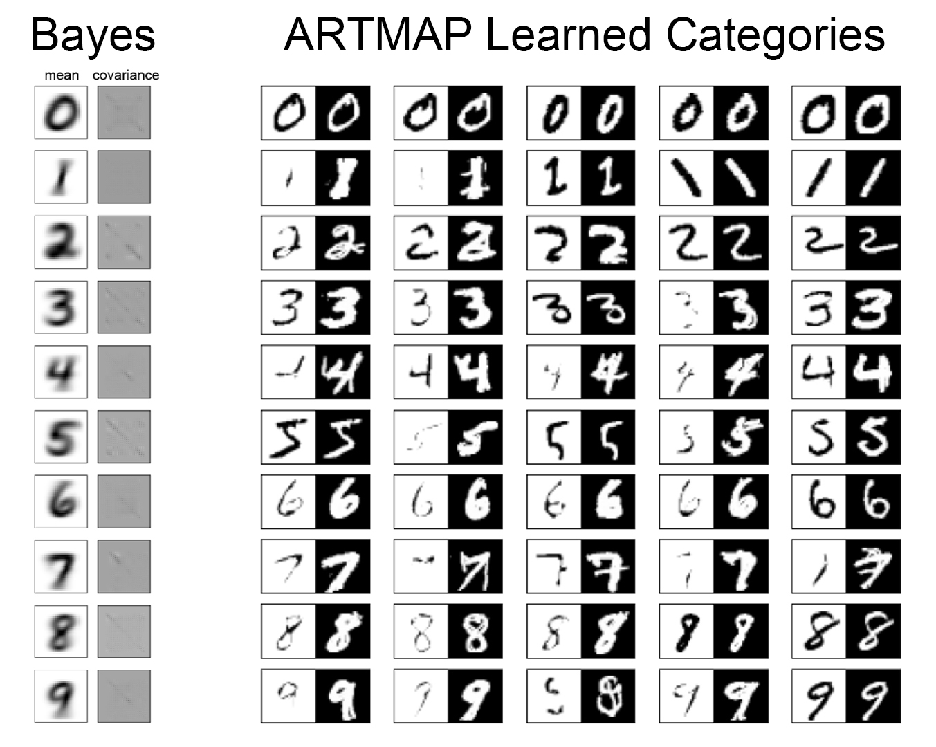
Figure 7: Internal model representations for Bayes and Fuzzy ARTMAP models. For Bayes, we are showing the class means (28x28 images) and covariance matrices (784x784). For Fuzzy ARTMAP, we are showing 5 representative Learned Category images for each class, using ARTMAP Complement Coding, in which each Learned Category is represented by the a bounding hypercuboid in 28x28=784 dimensional space, and the image shows the bottom left and upper right corners of the bounding hypercuboid, where the upper right corner is Complement-Coded, i.e. intensity_out = 1 - intensity_in.

• Manhattan and Euclidean Nearest Neighbor Classifiers get accuracy=96.3% and 96.9%, respectively. These are limiting cases of Fuzzy ARTMAP for Vigilance rho=1.0. They have zero training time because the model consists of the entire training dataset and a simple distance calculation rule. But their storage requirements are unreasonably large (60,000 x 784 = 47,040,000 parameters), so they are not used in practice.
• Bayesian Classifier gets accuracy=94.7%. The Bayesian Classifier computes the mean and covariance matrices for all the data in each class, and models each class with a Normal Distribution (Gaussian or Bell-shaped curve). The means (28x28 pixels) and covariances (784x784 pixels) for each class are shown in Figure 7. But in this small plot, it is not possible to see the fine structure of the covariance maps, so they have been replotted in Figure 8, in a way that preserves the 28x28 2D structure of the data.

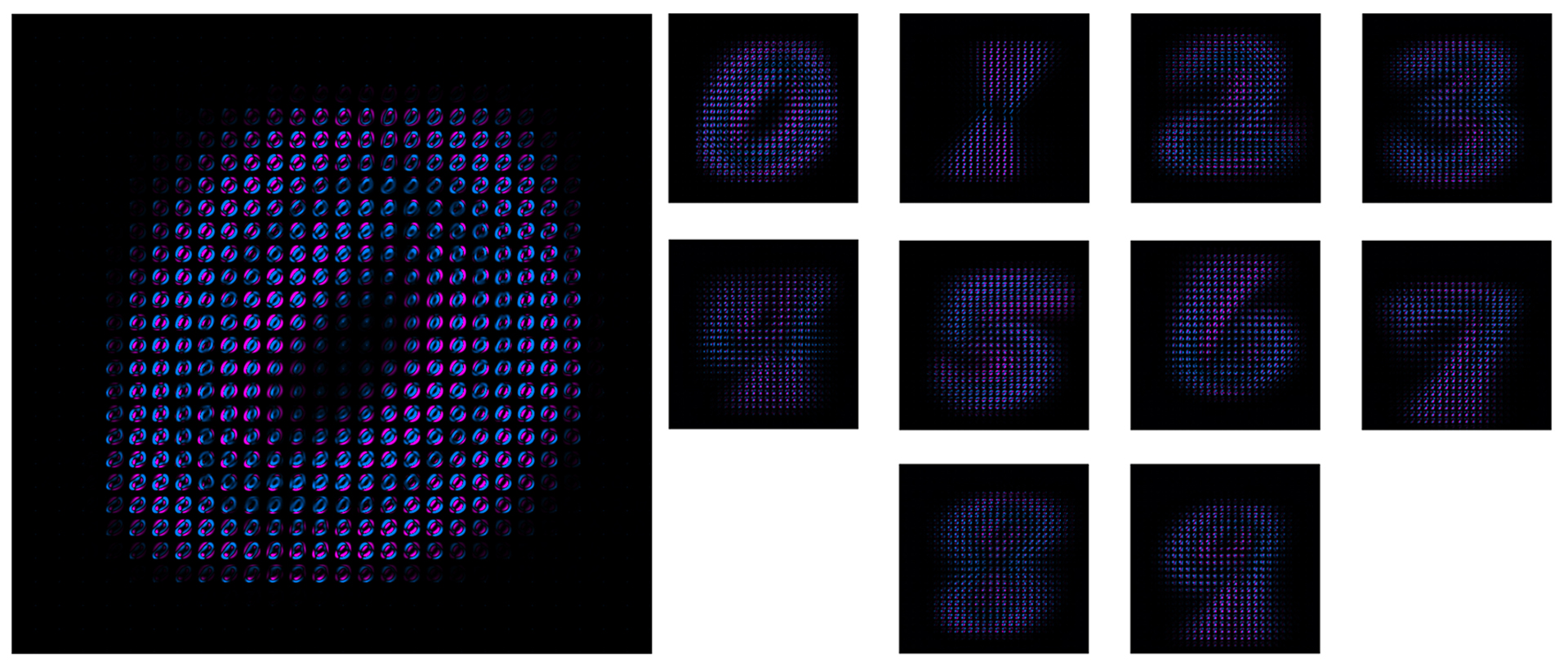
Figure 8: Bayes Covariance Maps for the MNIST digit classes. Normally these would be plotted as simple 784x784 covariance matrices. But that destroys the 28x28 structure. So, instead, we have plotted them as a 28x28 grid of 28x28 pixels. Plotted this way, the covariance matrix for the digit Zero looks like a big Zero made up of small center-surround Zeros. And similarly, the digit One looks like a big One made up of small Ones, etc. Bayesian Classifier is extremely fast to train, only 0.5s, because it only has to compute the means and covariance matrices of the training set. But it has rather poor accuracy=94.7%, because its model assumes a Gaussian distribution of the per-pixel data, and that is not a very good fit for the actual data distributions.

• Support Vector Machine with Radial Basis Function Kernel gets accuracy=98.36%. This is quite close to the best accuracy of 99.2% by the Deep Convolutional Neural Network.
• Deep Convolutional Neural Network gets accuracy=99.2%. This is the best-performing model on the MNIST task. But it has fairly long training time (4.4 minutes) over 14 training epochs, it is not capable of single-shot or few-shot learning, or Online continuous learning, and it is not inherently Explainable.
• Deep Convolutional Neural Network with Neocortix Deep Attribution Network gets accuracy=99.2%, and is Explainable. The Deep Attribution Network is trained to predict the index of the best training set sample, so the explanation for a given classification decision of a new test sample is that it is most similar to a known training sample of the same class. But this Explainability comes at the cost of much longer training duration (11.4 minutes) and very large storage requirements (20.4 Million parameters). In Figure 9, we show some examples of outputs of the Deep Attribution Network on MNIST samples.

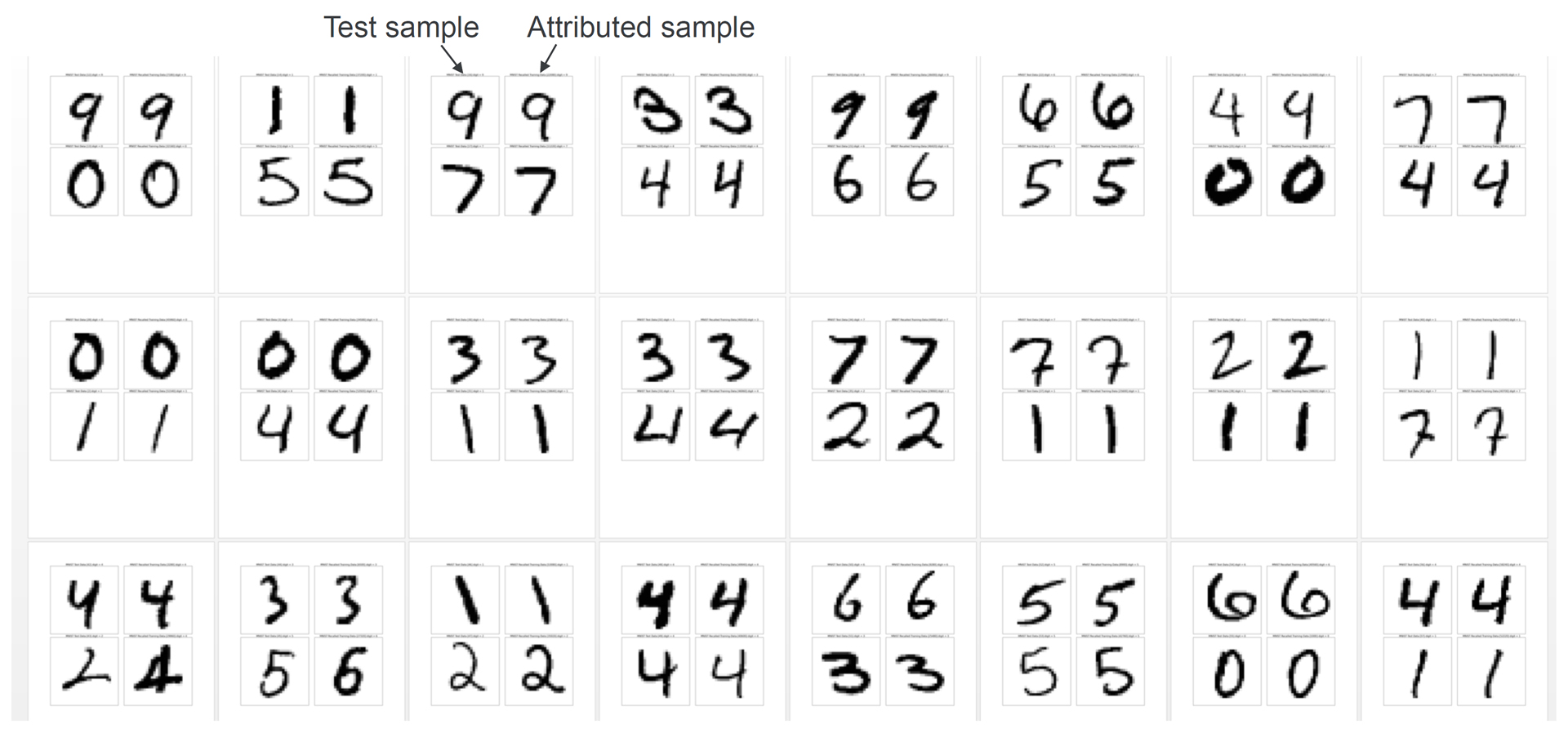
Figure 9: Examples of Deep Attribution Network Outputs for MNIST digit samples. For each new test sample, the Deep Attribution Network finds the index into the training set of the most similar training sample. The system can then retrieve and display the nearest training sample. Notice that the pairs of samples all have similar writing styles.

Visualizing MNIST Data

It would be great if we could visualize the MNIST training dataset, with its 60,000 28x28-pixel handwritten digit samples. If we could, we could then proceed to visualize the decision surfaces and decision boundaries of the different models, just as we did with the simple Circle-In-Square training dataset, and with this, we could really understand at a deep level how the different models work. But visualizing 60,000 data points in 10 classes in a 28x28=784-dimensional space is a hard problem in its own right. The best work I have seen on this fascinating problem is this 2014 blog post by Chris Olah, "Visualizing MNIST: An Exploration of Dimensionality Reduction", written when he was an intern at Google. I also recommend the original 2008 paper on the t-SNE method, by Laurens van der Maaten and Geoffrey Hinton, "Visualizing Data using t-SNE". "t-SNE" is an abbreviation of "t-Distributed Stochastic Neighbor Embedding".

In Figure 10, we show examples of MNIST t-SNE plots in 2 dimensions and 3 dimensions.

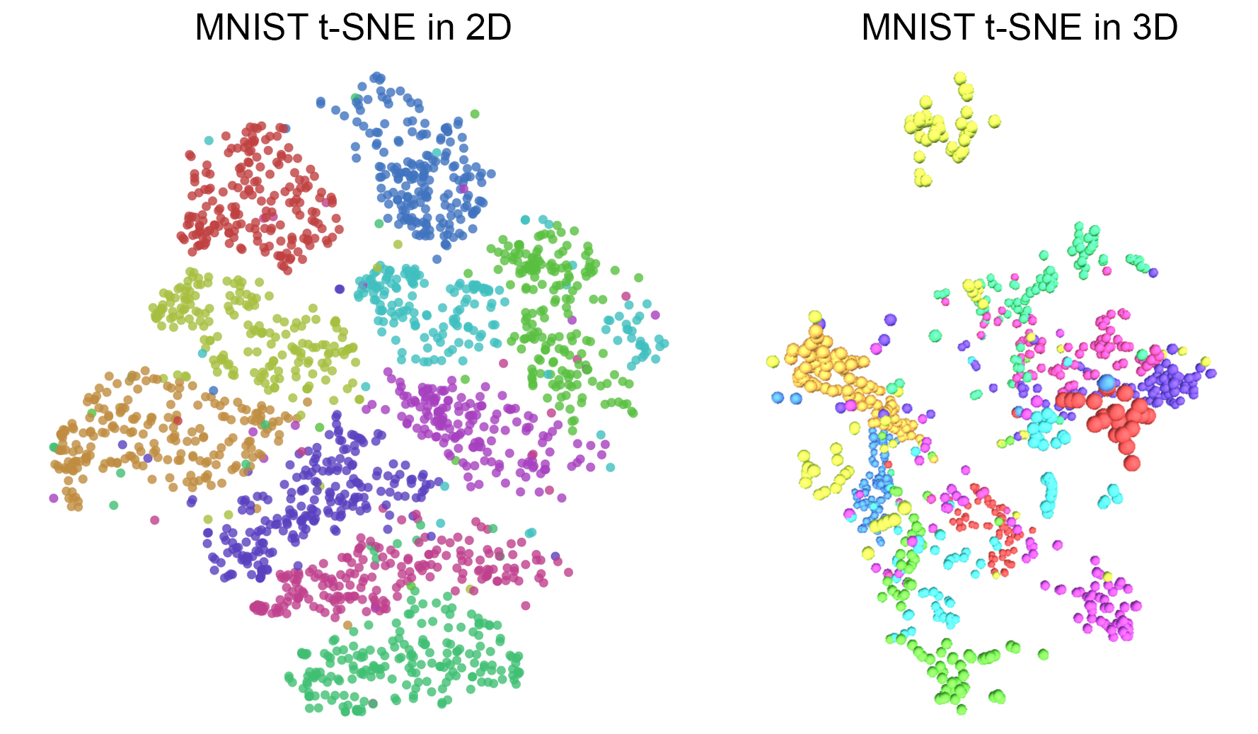
Figure 10: MNIST t-SNE Plots in 2 and 3 dimensions, from Chris Olah's blog. The colored dots represent training samples in the 10 different colored classes, projected from their original 784 dimensions into 2 or 3 dimensions, using the t-SNE transformation which preserves local Euclidean distances through the transformation.

The plots in Figure 10 illustrate that the t-SNE method does a good, but not perfect, job of transforming the data from the high-dimensional 784D space to the low-dimensional 2D or 3D space. There are some "stragglers", or data points which get separated from their main clusters. And, importantly, the 2D and 3D representations have some classes which do not have neighboring boundaries with other classes. Chris Olah summarized the final results: "If you want to visualize high dimensional data, there are, indeed, significant gains to doing it in three dimensions over two. There’s no way to map high-dimensional data into low dimensions and preserve all the structure. So, an approach must make trade-offs, sacrificing one property to preserve another."

So, 3 dimensions is better than 2 dimensions. This begs the question: would 4 dimensions be better than 3? It doesn't appear that anyone has tried a reduction to 4 dimensions, because we don't have good ways of visualizing data in 4D.

But Chris Olah mentioned another important idea in his blog, which he did not develop further: "People have lots of theories about what sort of lower dimensional structure MNIST, and similar data, have. One popular theory among machine learning researchers is the manifold hypothesis: MNIST is a low dimensional manifold, sweeping and curving through its high-dimensional embedding space."

Perhaps we can use all of the above ideas to make new progress on the problem. What if we represented the manifold as the surface of a 3D sphere? We have 10 classes (digits 0-9). Could we paint 10 regions on a 3D sphere, such that all 10 regions touch each other? I don't think it is possible. It's easy with 4 classes on a 3D sphere, with tetrahedral symmetry (like a tetrahedron, or pyramid). But even with 6 classes, with hexahedral symmetry (like a cube), it's not possible (opposite faces of a cube don't have a common edge).

But let's imagine we could pick a class, say 0, paint it red on the surface of a white sphere, and paint 9 colored wedges around it. That's a nice start, it shows the boundaries between Class 0 (red) and the other 9 classes. Now imagine we rotate the sphere in our hand so that we are looking straight at Class 1 (orange). We would like to see all the other 9 classes (0 and 2-9) arranged around Class1 (orange). Well, it's just not possible on a 3D sphere.

But with a higher-dimensional sphere, like 4D, I believe it is possible, and we can visualize it with series of rotated 2D views. The animation in Figure 11 below starts with Class 0 (red) at the center of all the other classes. And then it rotates Class 1 (orange) into the center, and all the other classes rotate to take their positions around Class 1. Similarly, we can keep rotating each Class into the center position, with the others arranged around the center class. With 10 rotational views, we can see each class surrounded by all of the others, with well-defined boundaries, with 10 2D images.

This simple way of looking at the data reduces the 10-Class 784-dimensional MNIST problem into 10 Binary 2-dimensional problems (with a very complicated mapping between them). It should be possible to use the t-SNE technique in this simplified space to plot the MNIST data.

Figure 11: MNIST: 10 Classes in 784 Dimensions Projected onto 4D Hypersphere. Each class has a boundary with all the other classes.

In Figure 11, we are representing the class regions as colored 2D shapes. But we can develop this idea further, to show the individual training samples as colored dots within those class regions. In Figure 12, we are visualizing the samples in each class as colored dots in a region on the surface of a 4D Hypersphere. It's not possible to view the full 4D Hypersphere surface in a single view, just like we can't see the whole surface of a sphere in a single view. For the MNIST example with 10 classes, we will have to rotate it 10 times to see the whole surface.

In the animation in Figure 12 below, we start with the rotation where the samples (red dots) of digit 0 are in the center region, surrounded by the samples (dots) of all the other digits (1-9). In this rotational view, the digit 0 region has a boundary with all the other digit regions. Next, we rotate to the view where the samples (orange dots) of digit 1 are in the center region, surrounded by the samples (dots) of all the other digits (0 and 2-9). In this rotational view, the digit 1 region has a boundary with all the other digit regions. Similarly, we can rotate a total of 10 times, bringing the samples of each digit into the center region, where it is surrounded by the samples of all the other digits.

This is a way of visualizing what a Machine Learning Classifier has to do. Given 60,000 labeled points in 784-dimensional space, it has to learn a mapping from 784-dimensions to 4 dimensions, so that all the points in each class remain in a contiguous group, and each group has a boundary with all the other groups. The conceptual method below shows how to start with the Manifold Hypothesis, pre-ordaining the 4D Hypersphere structure of the mapping, and then use t-SNE to place the points in the regions, with the constraint that the inter-point distances on the 4D Hypersphere manifold should be the same as the inter-point distances in the original 784-D space. This should result in an orderly, structured mapping of the MNIST training dataset to the 4D Hypersphere manifold.

Figure 12: MNIST: 10 Classes in 784 Dimensions Projected onto 4D Hypersphere, showing the data points in each class representing individual 28x28-pixel handwritten digit samples.

Finally, we have implemented the mapping from MNIST data points to the 4D Hypersphere manifold, for the view where Class 0 (red points) is at the center of the image, as shown in Figure 13. We used a novel constrained Multi-Dimensional Scaling algorithm, in which all the points in a given class all start in the same place in the 2D picture, and then the points move a little at each time step as though they have springs connecting them all, trying to pull them to the same distances observed in the 784-dimensional space. Over time, they move and settle into positions in 2D space that match the distances in 784-dimensional space, subject to the constraint that the points have to stay in their respective regions.

Figure 13: Showing a single view of 1000 MNIST data points (100 data points per class), where the data points from Class 0 (red points) are in the center of the image, using a novel constrained Multi-Dimensional Scaling method.

Conclusions

We have examined a number of popular Machine Learning methods, including Deep Neural Networks, Support Vector Machines, Adaptive Resonance Theory (ARTMAP), Bayesian Classifier, Manhattan and Euclidean Nearest Neighbor Classifiers, and Neocortix Deep Attribution Networks. We have applied those models to the simplest 2-dimensional 2-class Circle-In-Square problem, and the more complex 784-dimensional 10-class MNIST Handwritten Digits problem. We have shown how to visualize the training data, decision surfaces and decision boundaries of each method in the Circle-In-Square problem. We have measured the performance of each method on the MNIST problem, including accuracy, training and test duration, explainability, and capacity for online continuous learning. We have shown that when Explainability is achieved, it comes at a cost of additional parameter storage and training time. And we have shown conceptually how to visualize the 784-dimensional 10-class MNIST training data as a collection of 10 2-dimensional views, representing a 3D manifold on a 4D Hypersphere, suitable for mapping the individual training set data points with a novel constrained MDS method.

References

• Anthropic Interpretability Research, led by Chris Olah, 2025.
• "Visualizing MNIST: An Exploration of Dimensionality Reduction", blog by Chris Olah, 2014.
• "Visualizing Data using t-SNE", by Laurens van der Maaten and Geoffrey Hinton, 2008.